OpenPIV tutorial

In this tutorial we read a pair of images and perform the PIV using a standard algorithm. At the end, the velocity vector field is plotted.

from openpiv import tools, pyprocess, validation, filters, scaling

import numpy as np
import matplotlib.pyplot as plt
%matplotlib inline

import imageio
import importlib_resources
import pathlib

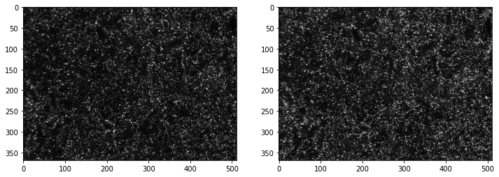
Reading images:

The images can be read using the imread function, and diplayed with matplotlib.

path = importlib_resources.files('openpiv')

frame_a  = tools.imread( path / 'data/test1/exp1_001_a.bmp' )
frame_b  = tools.imread( path / 'data/test1/exp1_001_b.bmp' )

fig,ax = plt.subplots(1,2,figsize=(12,10))
ax[0].imshow(frame_a,cmap=plt.cm.gray);
ax[1].imshow(frame_b,cmap=plt.cm.gray);

Processing

In this tutorial, we are going to use the extended_search_area_piv function, wich is a standard PIV cross-correlation algorithm.

This function allows the search area (search_area_size) in the second frame to be larger than the interrogation window in the first frame (window_size). Also, the search areas can overlap (overlap).

The extended_search_area_piv function will return three arrays. 1. The u component of the velocity vectors 2. The v component of the velocity vectors 3. The signal-to-noise ratio (S2N) of the cross-correlation map of each vector. The higher the S2N of a vector, the higher the probability that its magnitude and direction are correct.

winsize = 32 # pixels, interrogation window size in frame A
searchsize = 38  # pixels, search area size in frame B
overlap = 17 # pixels, 50% overlap
dt = 0.02 # sec, time interval between the two frames

u0, v0, sig2noise = pyprocess.extended_search_area_piv(
    frame_a.astype(np.int32),
    frame_b.astype(np.int32),
    window_size=winsize,
    overlap=overlap,
    dt=dt,
    search_area_size=searchsize,
    sig2noise_method='peak2peak',
)

The function get_coordinates finds the center of each interrogation window. This will be useful later on when plotting the vector field.

x, y = pyprocess.get_coordinates(
    image_size=frame_a.shape,
    search_area_size=searchsize,
    overlap=overlap,
)

Post-processing

Strictly speaking, we are ready to plot the vector field. But before we do that, we can perform some convenient pos-processing.

To start, lets use the function sig2noise_val to get a mask indicating which vectors have a minimum amount of S2N. Vectors below a certain threshold are substituted by NaN. If you are not sure about which threshold value to use, try taking a look at the S2N histogram with:

plt.hist(sig2noise.flatten())

invalid_mask = validation.sig2noise_val(
    sig2noise,
    threshold = 1.05,
)

Another useful function is replace_outliers, which will find outlier vectors, and substitute them by an average of neighboring vectors. The larger the kernel_size the larger is the considered neighborhood. This function uses an iterative image inpainting algorithm. The amount of iterations can be chosen via max_iter.

u2, v2 = filters.replace_outliers(
    u0, v0,
    invalid_mask,
    method='localmean',
    max_iter=3,
    kernel_size=3,
)

Next, we are going to convert pixels to millimeters, and flip the coordinate system such that the origin becomes the bottom left corner of the image.

# convert x,y to mm
# convert u,v to mm/sec

x, y, u3, v3 = scaling.uniform(
    x, y, u2, v2,
    scaling_factor = 96.52,  # 96.52 pixels/millimeter
)

# 0,0 shall be bottom left, positive rotation rate is counterclockwise
x, y, u3, v3 = tools.transform_coordinates(x, y, u3, v3)

Results

The function save is used to save the vector field to a ASCII tabular file. The coordinates and S2N mask are also saved.

tools.save('exp1_001.txt' , x, y, u3, v3, invalid_mask)

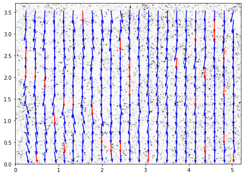
Finally, the vector field can be plotted with display_vector_field.

Vectors with S2N bellow the threshold are displayed in red.

fig, ax = plt.subplots(figsize=(8,8))
tools.display_vector_field(
    pathlib.Path('exp1_001.txt'),
    ax=ax, scaling_factor=96.52,
    scale=50, # scale defines here the arrow length
    width=0.0035, # width is the thickness of the arrow
    on_img=True, # overlay on the image
    image_name= str(path / 'data'/'test1'/'exp1_001_a.bmp'),
);