OpenPIV masking tutorial
In this tutorial we focus on the two ways you can use image masking in OpenPIV.
Definitions:
- static mask - an image with regions that should not be processed are marked as 1 (white color in black and white image or True) and regions that are processed are unmasked (zeros, False)
- dynamic mask - every pair of images (frame A, B) are processed to find out the region that has to be masked, e.g. a fish body around which we want to analyze PIV vectors. An average mask is then applied to both frames and PIV analysis
OpenPIV uses these masks in two ways:
- masked image regions are set to zero or completely black.
frame_a[image_mask] = 0 - PIV analysis in a completely black interrogation windows result in a zero peak and marked as invalid.
- in addition, the image mask is converted in a set of
x,ycoordinates on a PIV grid that mark the masked region in the vector field. Thesemask_coordsare propagating through the window deformation and stored with thex,y,u,v,maskin the ASCII result files. The vector fieldsu,varenumpy.MaskedArrayso the masked regions are invalid and should not appear in the plot. They could be also replaced by zeros orNaNif needed.
[1]:
from openpiv import tools, pyprocess, validation, filters, scaling, preprocess
import numpy as np
import matplotlib.pyplot as plt
%matplotlib inline

import imageio
import importlib_resources
import pathlib
[2]:
path = importlib_resources.files('openpiv') # pathlib.Path type
[3]:
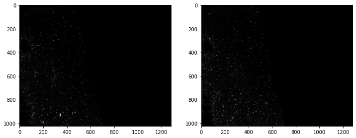
frame_a  = tools.imread( path / 'data' / 'test3' / 'pair_4_frame_0.jpg' )
frame_b  = tools.imread( path / 'data' / 'test3' / 'pair_4_frame_1.jpg' )
[4]:
fig,ax = plt.subplots(1,2,figsize=(12,10))
ax[0].imshow(frame_a,cmap='gray');
ax[1].imshow(frame_b,cmap='gray');
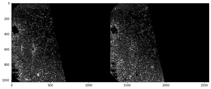
Rescale intensity or stretch histogram to get better contrast
[5]:
frame_a = preprocess.contrast_stretch(frame_a)
frame_b = preprocess.contrast_stretch(frame_b)
plt.figure(figsize=(12,12))
plt.imshow(np.c_[frame_a, frame_b], cmap='gray')
[5]:
<matplotlib.image.AxesImage at 0x7fec92ebf970>
Processing
In this tutorial, we are going to use the extended_search_area_piv function, wich is a standard PIV cross-correlation algorithm.
This function allows the search area (search_area_size) in the second frame to be larger than the interrogation window in the first frame (window_size). Also, the search areas can overlap (overlap).
The extended_search_area_piv function will return three arrays. 1. The u component of the velocity vectors 2. The v component of the velocity vectors 3. The signal-to-noise ratio (S2N) of the cross-correlation map of each vector. The higher the S2N of a vector, the higher the probability that its magnitude and direction are correct.
[6]:
winsize = 64 # pixels, interrogation window size in frame A
searchsize = 64  # pixels, search area size in frame B
overlap = 32 # pixels, 50% overlap
dt = 1.0 # sec, time interval between the two frames

u, v, sig2noise = pyprocess.extended_search_area_piv(
    frame_a.astype(np.int32),
    frame_b.astype(np.int32),
    window_size=winsize,
    overlap=overlap,
    dt=dt,
    search_area_size=searchsize,
    sig2noise_method='peak2peak',
)
The function get_coordinates finds the center of each interrogation window. This will be useful later on when plotting the vector field.
[7]:
x, y = pyprocess.get_coordinates(
    image_size=frame_a.shape,
    search_area_size=searchsize,
    overlap=overlap,
)
Post-processing
Strictly speaking, we are ready to plot the vector field. But before we do that, we can perform some convenient pos-processing.
To start, lets use the function sig2noise_val to get a mask indicating which vectors have a minimum amount of S2N. Vectors below a certain threshold are substituted by NaN. If you are not sure about which threshold value to use, try taking a look at the S2N histogram with:
plt.hist(sig2noise.flatten())
[8]:
flags = validation.sig2noise_val(
    sig2noise,
    threshold = 1.0
)
Another useful function is replace_outliers, which will find outlier vectors, and substitute them by an average of neighboring vectors. The larger the kernel_size the larger is the considered neighborhood. This function uses an iterative image inpainting algorithm. The amount of iterations can be chosen via max_iter.
[9]:
u, v = filters.replace_outliers(
    u, v,
    flags,
    method='localmean',
    max_iter=10,
    kernel_size=2,
)
Next, we are going to convert pixels to millimeters, and flip the coordinate system such that the origin becomes the bottom left corner of the image.
[10]:
# convert x,y to mm
# convert u,v to mm/sec

xs, ys, us, vs = scaling.uniform(
    x, y, u, v,
    scaling_factor = 96.52,  # 96.52 pixels/millimeter
)

# 0,0 shall be bottom left, positive rotation rate is counterclockwise
xs, ys, us, vs = tools.transform_coordinates(xs, ys, us, vs)
Results
The function save is used to save the vector field to a ASCII tabular file. The coordinates and S2N mask are also saved.
[11]:
# tools.save(filename, x,y,u,v, image_grid_mask, invalid_flag)
tools.save('exp1_001.txt', xs, ys, us, vs, flags)
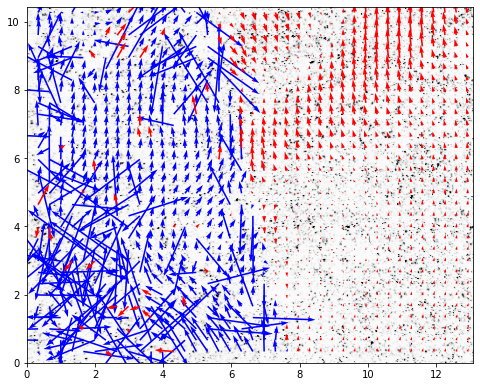
Finally, the vector field can be plotted with display_vector_field.
Vectors with S2N bellow the threshold are displayed in red.
[12]:
fig, ax = plt.subplots(figsize=(8,8))
tools.display_vector_field(
    pathlib.Path('exp1_001.txt'),
    ax=ax, scaling_factor=96.52,
    scale=2, # scale defines here the arrow length
    width=0.0035, # width is the thickness of the arrow
    on_img=True, # overlay on the image
    image_name= str(path / 'data'/'test1'/'exp1_001_a.bmp'),
);
If we do not want to show the invalid vectors
set show_invalid = False
[13]:
fig, ax = plt.subplots(figsize=(8,8))
tools.display_vector_field(
    pathlib.Path('exp1_001.txt'),
    ax=ax, scaling_factor=96.52,
    scale=2, # scale defines here the arrow length
    width=0.0035, # width is the thickness of the arrow
    on_img=True, # overlay on the image
    image_name= str(path / 'data'/'test1'/'exp1_001_a.bmp'),
    show_invalid=False,
);

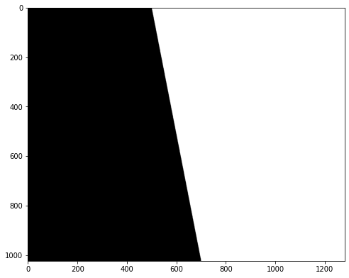
Tutorial on how to create a polygon mask
Start with drawing a polygon, use image coordinates
Important if the polygon touches borders, leave 5 pixels at least from the border
[14]:
from skimage.draw import polygon

fig, ax = plt.subplots(figsize=(8,8))

img = 0*frame_a.copy()


# ax.imshow(img, cmap='gray')

rr, cc = polygon(
    [0,frame_a.shape[0]-1,frame_a.shape[0]-1,0],
    [500,700,frame_a.shape[1]-1,frame_a.shape[1]-1]
 )
img[rr, cc] = 1

ax.imshow(img, cmap='gray')
[14]:
<matplotlib.image.AxesImage at 0x7fec92cbd2b0>
[15]:
# convert img to a boolean mask
img = np.where(img, True, False)
[16]:
# Note that mask_coordins for polygon are in image coordinates
# and here we need the grid coordinates, so we exchange x,y

# grid_mask = preprocess.prepare_mask_from_polygon(x, y, np.array(mask_coords)[:,::-1])

grid_mask = preprocess.prepare_mask_on_grid(x,y,img)
Now use the grid mask to create masked arrays, like in windef.py
[17]:
masked_u = np.ma.masked_array(u, mask=grid_mask)
masked_v = np.ma.masked_array(v, mask=grid_mask)
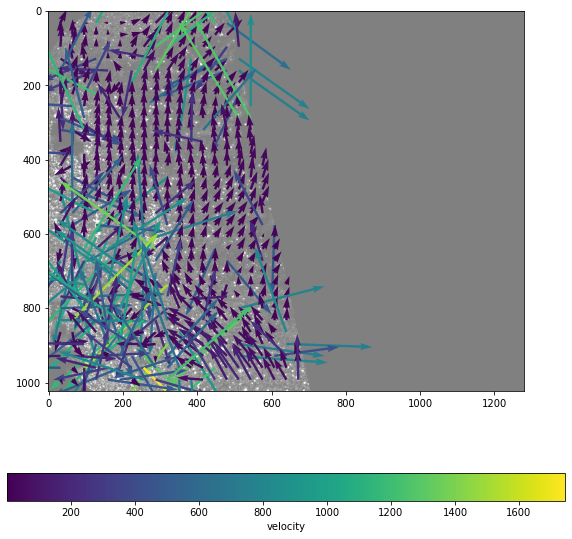
[28]:
fig, ax = plt.subplots(figsize=(10,10))
ax.imshow(frame_a, alpha=.5,cmap='gray',origin='lower')
Q = ax.quiver( x, y, masked_u, -masked_v, masked_u**2+masked_v**2, scale=150, width=.005,)
ax.invert_yaxis()
cb = fig.colorbar(Q,orientation='horizontal')
cb.set_label('velocity')
[ ]: